Archive
Money, Commodities, Balls, and How Much Deflation is Enough?
Money: How Much Deflation is Enough?
Once again, we see that the cure for all of the world’s ills is quantitative easing. Since there is apparently no downside to QE, it is a shame that we didn’t figure this out earlier. The S&P could have been at 200,000, rather than just 2,000, if only governments and central banks had figured out a century ago that running large deficits, combined with having a central bank purchase large amounts of that debt in the open market, was the key to rallying assets without limit.
That paragraph is obviously tongue-in-cheek, but on a narrow time-scale it really looks like it is true. The Fed pursued quantitative easing with no yet-obvious downside, and stocks blasted off to heights rarely seen before; the Bank of Japan’s QE has added 94% to the Nikkei in the slightly more than two years since Abe was elected; and today’s announcement by the ECB of a full-scale QE program boosted share values by 1-2% from Europe to the United States.
The ECB’s program, to be sure, was above expectations. Rather than the €50bln per month that had been mooted over the last couple of days with little currency-market reaction, the ECB pledged €60bln. And they promised to continue until September 2016, making the total value of QE around €1.1 trillion. (That’s about $1.3 trillion at today’s exchange rate, but of course if it works then it will be much less than $1.3 trillion at the September 2016 exchange rate). To be sure, a central bank always has the prerogative to change its mind, but on the risks of a sudden change in policy please see “Swiss National Bank”. It really is remarkable that Draghi was able to drag the Bundesbank kicking and screaming into this policy choice, and it is certain to end the threat of primary deflation in Europe just as it did in the U.S. and in Japan. It will likely also have similar effects on growth, which is to say “next to nothing.” But in Europe, deflation risks stemming from slow money growth had been a risk (see chart, source Bloomberg).

Interestingly, y/y money growth had already been accelerating as of late last year – the ECB releases M2 with a very long lag – but this puts the dot on the exclamation point. The ECB has said “enough!” There will be no core deflation in Europe.
Commodities: How Much Deflation is Enough?
Last week, in “Commodities Re-Thunk” and “Little Update on Commodities Re-Thunk”, I presented the results of using a generalization of the Erb & Harvey approach to forecast expected long-term real returns for commodities. It occurred to me that, since I have previously played with long-term real equity returns, and we have the real yield on 10-year TIPS as well, that it would be interesting to see if using these figures might produce a useful strategy for switching between assets (which doesn’t change the fact that I am a long-term investor; this is still based on long-term values. We merely want to put our assets in whatever offers the best long term value at the moment so as to maximize our expected long-term return).
The answer is yes. Now, I did a more-elegant version of what I am about to show, but the chart below shows the results of switching 100% of your assets between stocks, commodities, and TIPS based on which asset class had the highest expected real yield at a given month-end. Each line is an asset class, except for the blue line which shows the strategy result.

The labels at the top show the asset class that dominated for a long period of time. In 2005 there were a couple of quick crossovers that had little impact, but by and large there were three main periods: from 1999-2005, commodities offered excellent expected real returns; from mid-2005 through early-2008 the strategy would have been primarily in TIPS, and subsequent to that the strategy would have been primarily in equities. Fascinating to me is that the overall strategy does so well even though it would have been invested in equities throughout the crash in 2008. The crash in commodities was worse.
Now what is really interesting is that there is a vertical line at the far right-hand side of the chart. That is because at the end of December, the expected real return to commodities finally exceeded that of equities for the first time in a very long time. For this “selling out” strategy, that means you should be entirely out of stocks and TIPS and entirely in commodities.
As I said, that is the coarse version of this approach. My more-elegant version optimized the portfolio to have a constant expected risk in real terms. It was much less risky as a result (10.5% annualized monthly standard deviation compared to 15.5% for the strategy shown above), had lower turnover, but still sported returns over this period of 9.5% compounded compared to 11.2% for the strategy above. I am not, in other words, suggesting that investors put 100% of their assets in commodities. But this method (along with lots of other signals) is now suggesting that it is time to put more into commodities.
Balls: How Much Deflation is Enough?
Being a football fan, I can’t keep from weighing in on one mystery about deflate-gate (incidentally, why do we need to put ‘gate’ on the end of every scandal? It wasn’t Water-gate, it was the Watergate Hotel that proved Nixon’s undoing. “Gate” is not a modifier). Really, this part isn’t such a mystery but I have seen much commentary on this point: “How did the balls get deflated during the game since they were approved before the game?”
The answer is really simple in the real world: the official picked up one of the balls, said “fine”, and put them back in the bag. He has a million things to do before the championship game and in years of refereeing he has probably never found even one ball out of spec. This sort of error happens everywhere there are low reject rates, and it’s why good quality control is very difficult. (Now, if you fired the ref every time a bad ball got through, you damn betcha those balls would be measured with NASA-like precision – which is perhaps a bad metaphor, since similar issues contributed to the Challenger disaster). The real mystery to me is: if the Patriots truly think they are the better team, why would they cheat, even a little? As with the CHF/EUR cross that we discussed yesterday, the downside is far worse than the gain on the upside.
Or, is it? The NFL will have a chance to establish the cost of recidivism in cheating. Maybe the Patriots were simply betting that the downside “tail” to their risky behavior was fairly short. If the NFL wants to put a stop to nickel-and-dime cheats, it can do that by dropping the hammer here.
Little Update on Commodity Re-Thunk
Reading some of the comments people have posted in various places, I thought it would make sense to spend the time to re-create the projected-index chart in the prior article, but using something approximating GSCI weights. The GSCI is production-weighted, which means it is very heavily energy-linked (I used 2008 weights just because they were the first ones I found: 78% energy, 10% agriculture, 6% industrial metals, 3% meats, 3% precious metals), yet I was comparing its 10-year real return to an equal-weighted “prediction.” How much does this change the picture?
As it happens, quite a bit. Here is the new chart (sourced: Enduring Investments).

Commodities Re-Thunk
I want to talk about commodities today.
To be sure, I have talked a lot about commodities over the last year. Below I reprise one of the charts I have run in the past (source: Bloomberg), which shows that commodities are incredibly cheap compared to the GDP-adjusted quantity of money. It was a great deal, near all-time lows this last summer…until it started creating new lows.

Such an analysis makes sense. The relative prices of two items are at least somewhat related to their relative scarcities. We will trade a lot of sand for one diamond, because there’s a lot of sand and very few diamonds. But if diamonds suddenly rained down from the sky for some reason, the price of diamonds relative to sand would plummet. We would see this as a decline in the dollar price of diamonds relative to the dollar price of sand, which would presumably be stable, but the dollar in such a case plays only the role of a “unit of account” to compare these two assets. The price of diamonds falls, in dollars, because there are lots more diamonds and no change in the amount of dollars. But if the positions were reversed, and there were lots more dollars, then the price of dollars should fall relative to the price of diamonds. We call that inflation. And that’s the reasoning behind this chart: over a long period of time, nominal commodities prices should grow with as the number of dollars increases.
Obviously, this has sent a poor signal for a while, and I have been looking for some other reasonable way to compute the expected return on commodities.[1] Some time ago, I ran across an article by Erb and Harvey called The Golden Dilemma (I first mentioned it in this article). In it was a terrific chart (their Exhibit 5) which showed that the current real price of gold – simply, gold divided by the CPI price index – is a terrific predictor of the subsequent 10-year real return to gold. That chart is approximately reproduced, albeit updated, below. The data in my case spans 1975-present.

The vertical line indicates the current price of gold (I’ve normalized the whole series so that the x-axis is in 2015 dollars). And the chart indicates that over the next ten years, you can expect something like a -6% annualized real return to a long-only position in gold. Now, that might happen as a result of heavy inflation that gold doesn’t keep up with, so that the nominal return to gold might still beat other asset classes. But it would seem to indicate that it isn’t a great time to buy gold for the long-term.
This chart was so magnificent and made so much sense – essentially, this is a way to think about the “P/E ratio” for a commodity” that I wondered if it generalized to other commodities. The answer is that it does quite well, although in the case of many commodities we don’t have enough history to fill out a clean curve. No commodities work as well as does gold; I attribute this to the role that gold has historically played in investors’ minds as an inflation hedge. But for example, look at Wheat (I am using data 1970-present).

There is lots of data on agricultural commodities, because we’ve been trading them lots longer. By contrast, Comex Copper only goes back to 1988 or so:

Copper arguably is still somewhat expensive, although over the next ten years we will probably see the lower-right portion of this chart fill in (since we have traded higher prices, but only within the last ten years so we can’t plot the subsequent return).
Now the one I know you’re waiting for: Crude oil. It’s much sloppier (this is 1983-present, by the way), but encouraging in that it suggests from these prices crude oil ought to at least keep up with inflation over the next decade. But do you know anyone who is playing oil for the next decade?

For the sake of space, here is a table of 27 tradable commodities and the best-fit projection for their next 10 years of real returns. Note that most of these fit a logarithmic curve pretty reasonably; Gold is rather the exception in that the historical record is more convex (better expectation from these levels than a pure fit would indicate; see above).

I thought it was worth looking at in aggregate, so the chart below shows the average projected returns (calculated using only the data available at each point) versus the actual subsequent real returns of the S&P GSCI Excess Return index which measures only the return of the front futures contract.

The fit is probably better in reality, because the actual returns are the actual returns of the commodities which were in the index at the time, which kept changing. At the beginning of our series, for example, I am projecting returns for 20 commodities but the 10-year return compares an index that has 20 commodities in 1998 to one that has 26 in 2008. Also, I simply equal-weighted the index while the S&P GSCI is production-weighted. And so on. But the salient point is that investing in spot commodities has been basically not pretty for a while, with negative expected real returns for the spot commodities (again, note that investing in commodity indices adds a collateral return plus an estimate 3-4% rebalancing return over time to these spot returns).
Commodities are, no surprise, cheaper than they have been in a long while. But what is somewhat surprising is that, compared to the first chart in this article, commodities don’t look nearly as cheap. What does that mean?
The first chart in this article compares commodities to the quantity of money; the subsequent charts compare commodities to the price level. In short, the quantity of money is much higher than has historically been consistent with this price level. This makes commodities divided by M2 look much better than commodities divided by the price level. But it merely circles back to what we already knew – that monetary velocity is very low. If money velocity were to return to historical norms, then both of these sets of charts would show a similar story with respect to valuation. The price level would be higher, making the real price of commodities even lower unless they adjusted upwards as well. (This is, in fact, what I expect will eventually happen).
So which method would I tend to favor, to consider relative value in commodities? Probably the one I have detailed here. There is one less step involved. If it turns out that velocity reverts higher, then it is likely that commodities real returns will be better than projected by this method; but this approach ignores that question.
Even so, a projected real return now of -2% to spot commodities, plus a collateral return equal to about 1.9% (the 10-year note rate) and a rebalancing return of 3-4% produces an expected real return of 2.9%-3.9% over the next decade. This is low, and lower than I have been using as my assumption for a while, but it is far higher than the expected real returns available in equities of around 1.2% annualized, and it has upside risk if money velocity does in fact mean-revert.
I will add one final point. This column is never meant to be a “timing” column. I am a value guy, which means I am always seen to be wrong at the time (and often reviled, which goes with the territory of being a contrarian). This says absolutely nothing about what the returns to commodities will be over the next month and very little about returns over the next year. But this analysis is useful for comparing other asset classes on similar long-term horizons, and for using useful projections of expected real returns in asset allocation exercises.
[1] In what follows, I will focus on the expected return to individual spot commodities. But remember that an important part of the expected return to commodity indices is in rebalancing and collateral return. Physical commodities should have a zero (or less) real return over time, but commodity indices still have a significantly positive return.
Winter is Coming … But Not Here, Not Yet
We began 2014 with the perspective that the economy was limping along, barely surviving. A recession looked possible simply because the expansion was long in the tooth, but there weren’t any signs of it yet. Equity markets were priced for robust growth, which was clearly not likely to happen, but commodities and fixed-income markets were priced for disaster which was also not likely to happen. The investing risks were clearly tilted against stocks and bonds, given starting valuations, but although the economic landscape appeared weak it was not horrible.
Beginning 2015, the economic news is much better – at least, domestically. Unemployment is back to near levels associated with mid-cycle expansions, although there are still far too many people not in the workforce and a still-disturbing number of people who say they “want a job now” and would take one if offered (see chart, source Bloomberg).

More encouraging still, commercial bank credit growth is back to near 8% y/y, which is consistent with the booms of the past 30 years (see chart, source FRB). And this number excludes peer-to-peer lending and other sorts of credit growth that occur outside of the commercial bank framework, which is likely additive on a multi-year time frame.

The dollar is up and commodities are down, both of which are good for the US economy generally although bad for some groups of course (notably the oil patch). But the US is a net consumer of commodities, so commodity bear markets are good for US growth.
Outside of the US, though, things are looking decidedly worse. Although European core inflation recently surprised on the high side, it is still only at 0.8% and with GrExit a real possibility it is very hard to get bullish economically on the continent. China’s growth is softening. Emerging markets are not behaving well, especially the dollarized economies.
This recent development of the US as an island of relative tranquility in a sea of disquiet is interesting to me. Why are interest rates in the US so low, given that our economy is growing? 30-year interest rates at 2.5% and 10-year rates at 1.90%, with core inflation at 1.7% (and median inflation, as I like to point out because it isn’t influenced by outliers, at 2.3%) seems dissonant as the economy grows at 2.5%-3% and inflation in the US seems reasonably floored in the long run at 1.5%-2.0% as long as the Fed is credible.
This isn’t a new phenomenon, but I think the causes are new. Over the last five years, nominal interest rates were lower than they ought otherwise have been because the Fed was buying trillions of Treasuries and squeezing investors who needed to own fixed income. But the Fed is no longer buying and the Treasury is still issuing them. So I believe the causes of low interest rates now are different than the causes were over the last half-decade. Specifically, the causes of low interest rates in the last five years were sluggish global growth and extensive central bank QE; the causes currently are flight-to-quality related.
It seems weird to talk about a “flight to quality” in US bonds without stocks also plunging. But we have an analog for this period. Here is where I depart totally into intuition, which is in this case driven by experience. This period of interest rates declining while growth rises, as the economy continues a rebound after a long recession, with commodities declining and stocks rising, feels to me like late 1997. It feels like “Asian Contagion.”
Back in 1997, there was a lot of concern about how the Asian financial crisis would spill into US markets. Rates dropped (100bps in the 10y between July 1, 1997 and January 12, 1998), commodities dropped (the index now known as the Bloomberg Commodity Index fell 25% between October 1997 and June 1998), the S&P rallied (+23% from November 1997-April 1998), and GDP growth printed 5.2%, 3.1%, 4.0%, and 3.9% from 1997Q3 to 1998Q3. Meanwhile, Asian markets and economies were all but collapsing.
There was much fear at the time about the impact that the Asian Contagion would have on the US, but this country never caught a cold partly because (a) interest rates were depressed by the flight-to-quality and (b) declining commodities, especially energy, are bullish for US growth overall. We did not, of course, escape unscathed – later in 1998, a certain large hedge fund (which was small compared to some hedge funds today) threatened to cause large losses at some money center banks, and the Fed stepped in to save the day. That was a painful period in the equity market, but the effect from the Asian crisis was indirect rather than direct.
The parallels aren’t perfect; for one thing, bond yields are much lower and equity multiples much higher than their equivalents of the time, and commodities had already fallen very far before the recent slide. I would be reluctant to expect another hundred basis point rally in bonds and another large rally in stocks from these levels, although 1997-1999 saw these things. But history doesn’t repeat – it rhymes. I seem to hear this rhyme today.
Why does it matter? I think it matters because if I am right it means we are witnessing the end of long-term crisis-related markets, but they are masked by the arrival of short-term crisis-related markets. This means the unwind that we would have expected from the Fed’s ending of the purchase program – a slow return to normalcy – might instead end up looking like the unwind that we can get from short-term flight-to-quality crisis flows, which can be much more rapid. Again, this is all speculation and intuition, and I present no proof that I am right. I am merely proposing this speculation for my readers’ consumption and consideration.
Seasonal Allergies
Come get your commodities and inflation swaps here! Big discount on inflation protection! Come get them while you can! These deals won’t last long!
Like the guy hawking hangover cures at a frat party, sometimes I feel like I am in the right place, but just a bit early. That entrepreneur knows that hangover cures are often needed after a party, and the people at the party also know that they’ll need hangover cures on the morrow, but sales of hangover cures are just not popular at frat parties.
The ‘disinflation party’ is in full swing, and it is being expressed in all the normal ways: beat-down of energy commodities, which today collectively lost 3.2% as front WTI Crude futures dropped to a 2-year low (see chart, source Bloomberg),

…10-year breakevens dropped to a 3-year low (see chart, source Bloomberg),

…and 1-year inflation swaps made their more-or-less annual foray into sub-1% territory.

So it helps to remember that none of the recent thrashing is particularly new or different.
What is remarkable is that this sort of thing happens just about every year, with fair regularity. Take a look at the chart of 10-year breakevens again. See the spike down in late 2010, late 2011, and roughly mid-2013. It might help to compare it to the chart of front Crude, which has a similar pattern. What happens is that oil prices follow a regular seasonal pattern, and as a result inflation expectations follow the same pattern. What is incredible is that this pattern happens with 10-year breakevens, even though the effect of spot oil prices on 10-year inflation expectations ought to be approximately nil.
What I can tell you is that in 12 of the last 15 years, 10-year TIPS yields have fallen in the 30 days after October 15th, and in 11 of the past 15 years, 10-year breakevens were higher in the subsequent 30 days.
Now, a lot of that is simply a carry dynamic. If you own TIPS right now, inflation accretion is poor because of the low prints that are normal for this time of year. Over time, as new buyers have to endure less of that poor carry, TIPS prices rise naturally. But what happens in heading into the poor-carry period is that lots of investors dump TIPS because of the impending poor inflation accretion. And the poor accretion is due largely to the seasonal movement in energy prices. The following chart (source: Enduring Investments) shows the BLS assumed seasonality in correcting the CPI tendencies, and the actual realized seasonal pattern over the last decade. The tendency is pronounced, and it leads directly to the seasonality in real yields and breakevens.

This year, as you can tell from some of the charts, the disinflation party is rocking harder than it has for a few years. Part of this is the weakening of inflation dynamics in Europe, part is the fear that some investors have that the end of QE will instantly collapse money supply growth and lead to deflation, and part of it this year is the weird (and frustrating) tendency for breakevens to have a high correlation with stocks when equities decline but a low correlation when they rally.
But in any event, it is a good time to stock up on the “cure” you know you will need later. According to our proprietary measure, 10-year real yields are about 47bps too high relative to nominal yields (and we feel that you express this trade through breakevens rather than outright TIPS ownership, although actual trade construction can be more nuanced). They haven’t been significantly more mispriced than that since the crisis, and besides the 2008 example they haven’t been cheaper since the early days (pre-2003) when TIPS were not yet widely owned in institutional portfolios. Absent a catastrophe, they will not get much cheaper. (Importantly, our valuation metric has generally “beaten the forwards” in that the snap-back when it happens is much faster than the carry dynamic fades).
So don’t get all excited about “declining inflation expectations.” There is not much going on here that is at all unusual for this time of year.
The Dollar and Commodities – Just Friends
The recent, aggressive ECB ease, combined with some mild Fed growls about increasing rates “at some point,” ought to be good news for the dollar against the Euro. And so it has been, although as you see in this weekly chart (source: Bloomberg) the weakening of the Euro has been (a) mild and (b) started more than a month before the ECB actually took action. (Note that the units here are dollars per Euro).

Even though the ECB did considerably more than expected, much of that was in the form of a promise; until the body takes concrete steps towards implementing some of the new QE forms, the decline in the Euro is likely to be relatively slow and steady. Similarly, although the Yen has stopped weakening in 2014, I expect that trend has further to go as long as the Bank of Japan doesn’t lose its nerve with easing. In any event, both of those central banks seem at the moment to be more dovish than the Fed, which augurs for dollar strength.
Is that bad for commodities? The conventional wisdom is that since many commodities trade in dollars, a strong dollar implies weak commodities and vice versa.
There is some support for this view. The chart below (source: Bloomberg) shows weekly levels of the dollar index versus the DJ-UBS index, going back to 1996 or so. The correlation is okay, at -0.725.

Note, though, that this is a correlation of levels. If you look at a correlation of changes, which is what you would need to use dollar movements as a trading model for commodities, it is effectively zero. (These two series aren’t lovers, moving together always, but just friends coming together to the same place from time to time). Moreover, the regression of levels says that commodities are currently 15% or so cheap – the red smudge on the chart shows the current levels (yet another way that commodities appear to be cheap). Finally, the beta is quite low: if the dollar index rose 20%, it would correlate with roughly a 20% decline in commodities…if commodities preserved the same level of cheapness. To be sure, that is a sizeable drop but a 20% rise in the dollar would put it at levels not seen in more than a decade.
In any event, be careful not to confuse the nominal dollar price of commodities with the real price (I’ve made this argument from time to time in many contexts – see for example here, here, and here). Although changing the value of the dollar will diminish the price of commodities in dollars relative to what they would otherwise would be, if the global price level rises then the price of commodities will rise with it – they just may rise less than they otherwise would. And, since commodities typically experience their highest inflation “beta” at the beginning of an increase in inflation, it is reasonable to expect that commodities’ rise will be enough to cause any dollar-inspired softness to be completely obscured.
You still want to be long commodities if we are in an inflationary upswing, regardless of what the Fed does. And, needless to say, I am somewhat skeptical that the Fed will do anything particularly aggressive on the tightening side!
The China Syndrome
The last month or two has provided a wonderful illustration of why a diversified commodity index is a better investment than an investment in any given commodity. Since mid-February, April Lean Hogs has rallied 23%. Since late January, May Wheat is up 23%. March Coffee is up 80%. Gold is up 9%. But Crude Oil is 6% off its highs. Copper is 12% off its highs (8% since Thursday). April Nat Gas was up 42% from November through late February, but has lost 10% since then.
This is great if you happened to be 100% in Coffee, and bad if you happened to be heavy into copper or RIO or BHP. But this sort of volatility and non-correlation is exactly where much of the return to commodity indices, over the long run, comes from. Later this month, commodity indices will sell coffee and buy copper, systematically buying low and selling high. This phenomenon is worth on average a couple of points of return per year.
Most commentators seem to be focusing on the precipitous decline in copper prices, supposedly because “Doc Copper” is supposed to be a good leading indicator of economic growth. But in this case, the behavior of copper is mostly due to quasi-panic over China’s recently flagging growth figures. Although China is not the only consumer of copper (although sometimes you might think so, from the news coverage), prices are set at the margin and if there was an actual recession in China as opposed to a modest slowdown, then this would push copper prices lower.
But that would be terrific for Europe and the U.S., because it would mean cheaper copper for us. Similarly, decreasing Chinese growth would relax some pressure on energy prices, which would also be a boon for the Western world. I think people forget that one of the key reasons the “Asian Contagion” from the 1997 Asian Financial Crisis never happened (U.S. growth “bottomed” at 4.1% in mid-1998 – a level it hasn’t reached since 2004) was not because of Federal Reserve action (from March 1997 until August 1998, the Fed Funds target never budged from 5.5%) but because commodity prices plunged from 1997 into 1999. The DJ-UBS index fell from around 128 one month before the Thai baht collapsed to 75 in the first quarter of 1999 (see chart, source Bloomberg).

Even worse (or better, depending on your perspective) was the decline in energy. Crude oil dropped 55%, from the $25 area at the beginning of 1997 to $11 by late 1998. That remains the lowest real price of U.S. oil recorded since 1946 (see chart, source Enduring Investments using data from Dow Jones and the Bureau of Labor Statistics).
 It may be impolitic to say so, but probably the single best thing that could happen to U.S. growth would be for Chinese growth to slow, pushing the price of important commodity prices lower. As a nation, we consume far more commodities than we produce, so lower input prices is a net positive.
However, I suspect this is much ado about nothing. Chinese growth, even if it slows, is likely to remain plenty hot enough to keep commodity prices from falling very much, even in real terms. Real commodity prices have been falling steadily since 2011 (which is why all of the talk about the “end of the commodity supercycle” a year ago was so humorous) until early this year, even while the amount of currency in circulation has steadily increased. It certainly seems to me as if we have priced commodities fairly conservatively, and they can probably withstand a growth slowdown in China as long as the country doesn’t enter a bona fide crisis.
A Growling Bear is Bad for Everyone
I was convinced last week that the stock markets, as well as the inflation markets, were underestimating the importance of the Ukrainian conflict. I thought that I had a little more time to write about that before the crisis came to a head, which turned out not to be true. However, it seems that markets are still underestimating the importance of the Ukrainian conflict.
About the best possible outcome at this point is that Putin stops with an annexation of the Russian equivalent of the Sudetenland, with the episode merely pointing out (again) the impotence of Western leaders to respond to Russian aggression but not actually damaging much besides our pride. Even in that case, to me this signals a dangerous new evolution in the development of Russia’s relationship with the West. But the worse cases are far worse.
The angry fist-shaking of the old democracies is moderately amusing; less amusing are the stupid threats being made about economic sanctions. Let us stop for a minute and review what the West imports from Russia.
According to this article from Miyanville (from early 2013), Russia is the world’s largest producer of chromium (30% of the world market), nickel (19%), and palladium (43%), and is the second-largest producer of aluminum (10%), platinum (12%), and zirconium (19%). It has the largest supply of natural gas (although we are gaining rapidly), the second largest supply of coal, and the 8th-largest endowment of crude oil. The Ukraine itself is the third largest exporter of corn and the sixth-largest exporter of wheat. Meanwhile, the top 10 exports to Russia include engines, aircraft, vehicles, meat, electronic equipment, plastics, live animals, and pharmaceuticals.
So, we are fundamentally exporting “nice to haves” while importing “must haves.” Who needs trade more?
Let me make a further, suggestive observation. I maintain that the tremendous, positive trade-off of growth and inflation (high growth, low inflation) that the U.S. has experienced since the 1990s is at least partly a story of globalization following the end of the Cold War. Over the last couple of years, I have grown fond of showing the graph of apparel prices, which shows a steady rise until the early 1990s, a decline until 2012 or so, and then what appears to be a resumption of the rise. The story with apparel is very clear – as we moved from primarily domestically-sourced apparel to almost completely overseas-sourced apparel, high-cost production was replaced by low-cost production, which dampened the price increases for American consumers. It is a very clear illustration of the “globalization dividend.”
Of course, mainstream economic theory holds that the inflation/growth tradeoff suddenly became attractive for the U.S. in 1991 or so because inflation expectations abruptly became “anchored.” Why look for a good reason, when you can simply add a dummy variable to an econometric model??
But suppose that I am right, and the fall of the Soviet Union in 1991 played a role in the terrific growth/inflation tradeoff we have experienced since then. Incidentally, here are some data:
- Cold War (1963, immediately following the Cuban missile crisis, until the fall of the USSR): U.S. annual growth averaged 3.4% (not compounded); inflation averaged 5.4%. The DJIA rose at a compounded nominal rate of 5.6%.
- Post-Cold-War (1991-2013, including three recessions): U.S. annual average growth 2.6%; annual average inflation 2.4%. The DJIA rose at a compounded nominal rate of 7.5%.
This is not to say that globalization is about to end, or go into reverse, necessarily. It is to illustrate why we really ought to be very concerned if it appears that the Bear appears to be back in expansion mode – whether it is something we can prevent or not. And it is also to illustrate why putting a firm end to that expansion mode, rather than sacrificing global trade and cheap energy to a resurrection of the Cold War, is probably worth considering.
I still don’t think that equity investors understand the significance of what is going on in the Ukraine.
The Marie Antoinette Rule
The biggest surprise of the day on Tuesday did not come from new Fed Chairman Janet Yellen, nor from the fact that she didn’t offer dovish surprises. Many observers had expected that after a mildly weak recent equity market and slightly soft Employment data, Yellen (who has historically been, admittedly, quite a dove) would hold out the chance that the “taper” may be delayed. But actually, she seemed to suggest that nothing has changed about the plan to incrementally taper Fed purchases of Treasuries and mortgages. I had thought that would be the likely outcome, and said so yesterday when I supposed “she will be reluctant to be a dove right out of the gate.”
The surprise came in the market reaction. Since there had been no other major (equity) bullish influences over the last week, I assumed that the stock market rally had been predicated on the presumption that Yellen would give some solace to the bulls. When she did not, I thought stocks would have difficulty – and on that, I was utterly wrong. Now, whether that means the market thinks Yellen is lying, or whether there is some other reason stocks are rallying, or whether they are rallying for no reason whatsoever, I haven’t a clue.
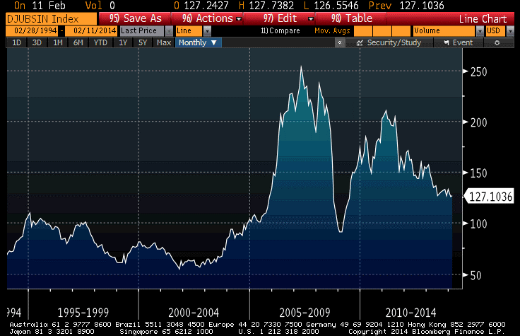
I do know though that the DJ-UBS commodity index reached its highest closing level in five months, and that commodities are still comfortably ahead of stocks in 2014 even with this latest equity rally. This rally has been driven by energy and livestock, with some precious metals improvements thrown in. So, lest we be tempted to say that the rally in commodities is confirming some underlying economic strength, reflect that industrial metals remain near 5-year lows (see chart, source Bloomberg, of the DJUBS Industrial Metals Subindex).
One of the reasons I write these articles is to get feedback from readers, who forward me all sorts of articles and observations related to inflation. Even though I have access to many of these same sources, I don’t always see every article, so it’s helpful to get a heads up this way. A case in point is the article that was on Business Insider yesterday, detailing another quirky inflation-related report from Goldman Sachs.http://www.businessinsider.com/goldman-fed-should-target-wage-growth-2014-2
Now, I really like much of what Jan Hatzius does, but on inflation the economics team at Goldman is basically adrift. It may be that the author of this article doesn’t have the correct story, but if he does then here is the basic argument from Goldman: the Fed shouldn’t target inflation or employment, but rather on wage growth, because wage growth is a better measure of the “employment gap” and will tie unemployment and inflation together better.
The reason the economists need to make this argument is because “price inflation is not very responsive to the employment gap at low levels of inflation,” which is a point I have made often and most recently in my December “re-blog” series.
But, as has happened so often with Goldman’s economists when it comes to inflation, they take a perfectly reasonable observation and draw a nonsensical conclusion from it. The obvious conclusion, given the absolute failure of the “employment gap” to forecast core price inflation over the last five years, is that the employment gap and price inflation are not particularly related. The experimental evidence of that period makes the argument that they are – which is a perversion of Phillips’ original argument, which related wages and unemployment – extremely difficult to support. Hatzius et. al. clearly now recognize this, but they draw the wrong conclusion.
There is no need to tie unemployment and inflation together …unless you are a member of the bow-tied set, and really need to calibrate parameters for the Taylor Rule. So it isn’t at all a concern that they aren’t, unless you really want your employment gap models to spit out useful forecasts. Okay, so if you can’t forecast prices, then use the same models and call it a wage forecast!
But the absurdity goes a bit farther. By suggesting that the Fed set policy on the basis of wage inflation, these economists are proposing a truly abhorrent policy of raising interest rates simply because people are making more money. Wage inflation is a good thing; end product price inflation is a bad thing. Under the Goldman rule, if wages were rising smartly but price inflation was subdued, then the Fed should tighten. But why tighten just because real wages are increasing at a solid pace? That is, after all, one of society’s goals! If the real wage increase came about because of an increase in productivity, or because of a decrease in labor supply, then it does not call for a tightening of monetary policy. In such cases, it is eminently reasonable that laborers take home a larger share of the real gains from manufacture and trade.
On the other hand, if low nominal wage growth was coupled with high price inflation, the Goldman rule would call for an easing of monetary policy…even though that would tend to increase price inflation while doing nothing for wages. In short, the Goldman rule should probably be called the Marie Antoinette rule. It will tend to beat down wage earners.
Whether or not the Goldman rule is an improvement over the Taylor Rule is not necessarily the right question either, because the Taylor Rule is not the right policy rule to begin with. Returning to the prior point: the employment gap has not demonstrated any useful predictive ability regarding inflation. Moreover, monetary policy has demonstrated almost no ability to make any impact on the unemployment rate. The correct conclusion here is a policy rule should not have an employment gap term. The Federal Reserve should be driven by prospective changes in the aggregate price level, which are in turn driven in the long run almost entirely by changes in the supply of money. So it isn’t surprising that the Goldman rule can improve on the Taylor rule – there are a huge number of rules that would do so.
Do Data Matter Again?
In normal times, by which I mean before actions of the Federal Reserve became the only data point that mattered, the monthly ISM report was important because it was the first broad-based look at the most-recent month’s data.
Now that the Fed’s taper has begun – right about the time that the uncertainty of the impact of Obamacare implementation was at its peak, curiously enough – the ISM data seems to have taken on importance once again. I must say that I did not see that coming, but since guessing at the Fed’s actions every six weeks and ignoring all intervening data was so all-fired boring, I suppose I am glad for it. Looking at economic data and trying to figure out what is happening in the economy is more like analysis and less like being on The People’s Court trying to rule on a he-said, she-said case where the hes and shes are Federal Reserve officials. And that is welcome.
That being said, the January ISM report isn’t one I would necessarily place at the head of the class of importance, mainly because it is January. Still, it was an interesting one with the Manufacturing PMI dropping 5.2 points, matching the steepest decline since October 2008. The New Orders subindex plunged to 51.2 versus 64.4 last month, and Employment and Production indices also declined significantly. It’s clearly bad news, but I would be careful ascribing too much value to any January number – especially one based on a survey.
Also standing out in the report was the increase in the (non-seasonally adjusted) “Prices Paid” subcomponent, to 60.5. the jump was initially somewhat surprising to me because as the chart below – which I tweeted shortly after the number – seems to show, we have had a jump in Prices Paid that is not being driven by a concomitant jump in gasoline prices – and Prices Paid is predominantly driven by gasoline prices.

However, as I noted in that tweet, the Prices Paid index is measuring the rate of change of prices (the question posed to purchasing managers is whether prices are increasing faster, slower, or about the same as the month before), so just eyeballing it may not be enough. The chart below plots the 3-month change in gasoline prices versus the ISM Prices Paid subindex. What you can see is that the first chart is slightly deceiving. The change in gasoline prices has accelerated – back to zero after having been declining since February of 2013. And “unchanged” gasoline prices is roughly consistent with about 60 on the Prices Paid indicator. So, this isn’t as much of a surprise as it looked like, initially.

Still, whether it was the data or because of continued concern about emerging markets (though the S&P fell nearly as far in percentage terms as did the EEM today, leaving open the question of which is following which), stocks didn’t enter February with much cheer. But never fear, I am sure there is “cash on the sidelines” that will come charging to the rescue soon.
The past week has given a great illustration of one important difference between the price behavior of equities and commodities. That is that stocks are negatively skewed and positively kurtotic, while commodities are positively skewed and negatively kurtotic. That is to say, in layman’s terms, that stocks tend to crash downward, while commodities more frequently crash upwards. This happens because what tends to drive severe movements in commodities is shortages, where the short-term supply curve becomes basically vertical so that any increase in demand pushes up prices sharply. Exhibit one is Natural Gas (see chart, source Bloomberg), where inventories were above normal as recently as October and now are the lowest in a decade.
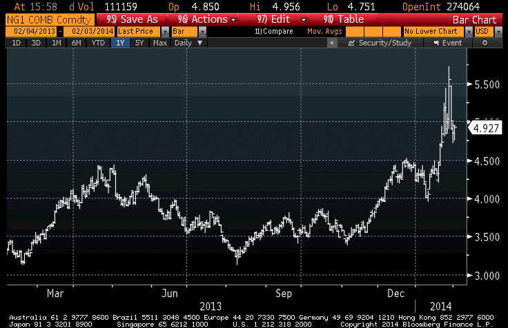
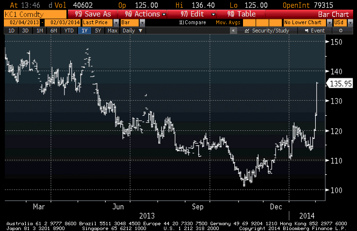
Exhibit two is Coffee (see chart, source Bloomberg), where drought in Brazil has lifted coffee prices 8-9% today and 35% from the five-year lows set in November. There’s an awful lot of coffee in Brazil, I understand, but there may be less this year.
In my view, stocks remain very expensive even after this quick 5.75% loss (-2.3% today). Obviously, less so! Commodities have outperformed stocks by basically remaining unchanged, but remain very cheap. Bonds have rallied, as money has shifted from stocks to bonds. This is fine, except that 10-year notes at 2.57% with median inflation at 2.1% and rising is not a position to own, only to rent. The question is, when investors decide that it’s time to take their profits in bonds, do they go to cash, back to equities, or to commodities? If you are one of the people mulling this very question, I have another chart to show you. It is the simple ratio of the S&P to the DJ-UBS (source: Bloomberg).

I think that makes where I stand fairly clear. If both stocks and commodities represent ownership in real property, and both have roughly the same long-term historical returns (according to Gorton & Rouwenhorst), then the ratio of current prices should be a coarse (and I stress coarse) relative-value indicator, right?
But let’s shift from the long-view lens back to the short view, now that a retreating Fed makes this more worthwhile. I am not sanguine about the outlook for stocks, obviously (and here’s one for the technicians: for the first time in years, exchange volume in January was higher than last year’s January volume). However, bulls may get a brief reprieve later this week when the Employment Report is released. Yes, it’s another January data point that ought to be ignored or at least averaged with December’s figure. And that’s the point here. Last month’s Employment Report showed only a 74k rise in Nonfarm Payrolls. That weakness was likely due to the fact that the seasonal adjustments (which dwarf the net number of jobs, in December and January) assumed more year-end and holiday hiring than actually occurred. But the flip side of that is that if fewer were hired in December, it probably means fewer were fired in January. Thus, I expect that the 185k consensus guess for new jobs is likely to be too low and we will have a bullish surprise on Friday. That might help the bulls get a foothold…but it is a long three trading days away.
