Archive
The Destination Currency in the Global Carry Trade: USD?
If you are an investor of the Ben Graham school, you’ve lived your life looking for “value” investments with a “margin of safety.” Periodically, if you are a pure value investor, then you go through long periods of pulling your hair out when momentum rules the day, even if you believe – as GMO’s Ben Inker eloquently stated in last month’s letter – that in the long run, no factor is as important to investment returns as valuation.
This is one of those times. Stocks have been egregiously overvalued (using the Shiller CAPE, or Tobin’s Q, or any of a dozen other traditional value metrics) for a very long time now. Ten-year Treasuries are at 1.80% in an environment where median inflation is at 2.5% and rising, and where the Fed’s target for inflation is above the long-term nominal yield. TIPS yields are significantly better, but 10-year real yields at 0.23% won’t make you rich. Commodities are very cheap, but that’s just a bubble in the other direction. The bottom line is that the last few years have not been a great time to be purely a value investor. The value investor laments “why?”, and tries to incorporate some momentum metrics into his or her approach, to at least avoid the value traps.
Well, here is one reason why: the US is the destination currency in the global carry trade.
A “carry trade” is one in which regular returns can be earned simply on the difference in yields between different instruments. If I can borrow at LIBOR flat and lend at LIBOR+2%, I am in a carry trade. Carry trades that are riskless and result from one’s market position (e.g., if I am a bank and I can borrow from 5-year CD customers at 0.5% and invest in 5-year Treasuries at 1.35%) are usually more like accrual trades, and are not what we are talking about here. We are talking about positions that imply some risk, even if it is believed to be small. For example, because we are pretty sure that the Fed will not tighten aggressively any time soon, we could simply buy 2-year Treasuries at 0.88% and borrow the money in overnight repo markets at 0.40% and earn 48bps per year for two years. This will work unless overnight interest rates rise appreciably above 88bps.
We all know that carry trades can be terribly dangerous. Carry trades are implicit short-option bets where you make a little money a lot of the time, and then get run over with some (unknown) frequency and lose a lot of money occasionally. But they are seductive bets since we all like to think we will see the train coming and leap free just in time. There’s a reason these bets exist – someone wants the other side, after all.
Carry trades in currency-land are some of the most common and most curious of all. If I borrow money for three years in Japan and lend it in Brazil, then I expect to make a huge interest spread. Of course, though, this is entirely reflected in the 3-year forward rate between yen and real, which is set precisely in this way (covered-interest arbitrage, it is called). So, to make money on the Yen/Real carry bet, you need to carry the trade and reverse the exchange rate bet at the end. If the Real has appreciated, or has been stable, or has declined only a little, then you “won” the carry trade. But all you really did was bet against the forward exchange rate. Still, lots and lots of investors make precisely this sort of bet: borrowing money is low-interest rate currencies, investing in high-interest-rate currencies, and betting that the latter currency will at least not decline very much.
How does this get back to the value question?
Over the last several years, the US interest rate advantage relative to Europe and Japan has grown. This should mean that the dollar is expected to weaken going forward, so that someone who borrows in Euro to invest in the US ought to expect to lose on the future exchange rate when they cash out their dollars. And indeed, as the interest rate advantage has widened so has the steepness of the forward points curve that expresses this relationship. But, because investors like to go to higher-yielding currencies, the dollar in fact has strengthened.
This flow is a lot like what happens to people on a ship that has foundered on rocks. Someone lowers a lifeboat, which looks like a great deal. So people begin to pour into the lifeboat, and they keep doing so until it ceases, suddenly, to be a good deal. Then all of those people start to wish they had stayed on the ship and waited for help.
In any event, back to value: the chart below (source: Bloomberg) shows the difference between the 10-year US$ Libor swap rate minus the 10-year Euribor swap rate, in white and plotted in percentage terms on the right-hand scale. The yellow line is the S&P 500, and is plotted on the left-hand scale. Notice anything interesting?

The next chart shows a longer time scale. You can see that this is not a phenomenon unique to the last few years.

Yes, the correlation isn’t perfect but to me, it’s striking. And we can probably do better. After all, the chart above is just showing the level of equity prices, not whether they are overvalued or undervalued, and my thesis is that the fact that the US is the high-yielding currency in the carry trade causes the angst for value investors. We can show this by looking at the interest rate spread as above, but this time against a measure of valuation. I’ve chosen, for simplicity, the Shiller Cyclically-Adjusted P/E (CAPE) (Source: http://www.econ.yale.edu/~shiller/data.htm)

Now, I should take pains to point out that I have not proven any causality here. It may turn out, in fact, that the causality runs the other way: overheated markets lead to tight US monetary policy that causes the interest rate spread to widen. I am skeptical of that, because I can’t recall many episodes in the last couple of decades where frothy markets led to tight monetary policy, but the point is that this chart is only suggestive of a relationship, not indicative of it. Still, it is highly suggestive!
The implication, if there is a causal relationship here, is interesting. It suggests that we need not fear these levels of valuation, as long as interest rates continue to suggest that the US is a good place to keep your money (that is, as long as you aren’t afraid of the dollar weakening). That, in turn, suggests that we ought to keep an eye on rates of change: if the ECB tightens more, or eases less, than is priced into European markets (which seems unlikely), or the Fed tightens less, or eases more, than is priced into US markets (which seems more likely, but not super likely since not much is presently priced in), or the dollar trend changes clearly. When one of those things happens, it will be a sign that not only are the future returns to equities looking unrewarding, but the more immediate returns as well.
Irrational Lugubriousness on Inflation
Today the 1-year CPI swap rate closed at 1.77%, the highest rate since 2014 (see chart, source Bloomberg).

The CPI swap (which, as an aside, is a better indicator of expected inflation than are breakevens, for technical reasons discussed here for people who truly have insomnia) indicates that headline inflation is expected to be about 1.77% over the next year. That’s nearly double the current headline inflation rate, but well below the Fed’s target of roughly 2.3% on a CPI basis. But at least on appearances, investors seem to be adjusting to the reality that inflation is headed higher.
Unfortunately, appearances can be deceiving. And in this case, they are. The headline inflation rate is of course the combination of core inflation plus food inflation and energy inflation; as a practical matter most of the volatility in the headline rate comes from the volatility endemic in energy markets. I’ve observed before that this leads to unreasonable volatility in long-term inflation expectations, but in short-term inflation expectations it makes perfect sense that they ought to be significantly driven by expectations for energy prices. The market recognizes that energy is the source of inflation volatility over the near-term, which is why the volatility curve for inflation options looks strikingly like the volatility curve for crude oil options and not at all like the volatility curve for LIBOR (see chart, source Enduring Investments).

The shape of the energy futures curves themselves also tell us what amount of energy price change we should include in our estimate of future headline inflation (or, alternatively, what energy price change we can hedge out to arrive at the market’s implied bet on core inflation). I am illustrating this next point with the crude oil futures curve because it doesn’t have the wild oscillations that the gasoline futures curve has, but in practice we use the gasoline futures since that is closer to the actual consumption item that drives the core-headline difference. Here is the contract chart for crude oil (Source: Bloomberg):

So, coarsely, the futures curve implies that crude oil is expected to rise about $4, or about 9%, over the next year. This will add a little bit to core inflation to give us a higher headline rate than the core inflation rate. Obviously, that might not happen, but the point is that it is (coarsely) arbitrageable so we can use this argument to back into what the market’s perception of forward core inflation is.
And the upshot is that even though 1-year CPI swaps are at the highest level since 2014, the implied core inflation rate has been steadily falling. Put another way, the rise in short inflation swaps has been less than the rally in energy would suggest it should have been. The chart below shows both of these series (source: Enduring Investments).

So – while breakevens and inflation swaps have been rallying, in fact this rally is actually weaker than it should have been, given what has been happening in energy markets. Investors, in short, are still irrationally lugubrious about the outlook for price pressures in the US over the next few years. Remember, core CPI right now is 2.2%. How likely is it to decelerate 1.5% or more over the next twelve months?
(**Administrative Note: Get your copy of my new book What’s Wrong with Money: The Biggest Bubble of All! Here is the Amazon link.)
Book Review: “Where Keynes Went Wrong”
Last week I mentioned something about what Keynes said in the General Theory, and promised to expand on that a bit this week. I will do so, in the form of a book review.
I can’t remember who it was, and I’m sorry, but one of the people who read my articles suggested a book to me a year or so ago published in 2009 and called Where Keynes Went Wrong: And Why World Governments Keep Creating Inflation, Bubbles, and Busts by Hunter Lewis, and I finally got around to reading it. I am very glad I did – this book is terrific, and is a must-read if you are either pro-Keynes or anti-Keynes.
Of course, readers will know from my articles that I am anti-Keynes, although more precisely I am anti-Keynesian in the modern sense of that word. I never read very much of the General Theory, because honestly it is poorly written in the sense of its prose, and I always assumed that Keynes probably had some great insights and it was the later Keynesians that screwed up what he said.
Oh, I was so wrong. Keynes was looney tunes. A bona fide lunatic. He proved masterful in manipulating the cult of personality that existed at the time he was writing, however; he was adept at destroying his opponents in ways that sounded erudite and like certain later personalities the media adored him. All of this is well-documented by Mr. Lewis, although the looney tunes conclusion is my own.
The book is put together brilliantly. The author quotes passages from Keynes, using actual quotes interspersed with paraphrasing – which is necessary because, as I said above, the General Theory is poorly written and opaque. But it isn’t the paraphrasing that is damning. When Mr. Lewis wants to indict Keynes, he does it with his own words. For example, in unraveling the absurd (and often self-contradictory) prescriptions that Keynes had for managing the macro economy, Mr. Lewis declares that Keynes thought government should never raise interest rates. That’s right, never.[1] But you needn’t take Lewis’ word for it. Here’s Keynes, cited in the book:
“The remedy for the boom is not a higher rate of interest but a lower rate of interest! For that may enable the boom to last. The right remedy for the trade cycle is not to be found in abolishing booms and thus keeping us permanently in a semi-slump; but in abolishing slumps and thus keeping us permanently in a quasi-boom.”[2]
If you are anything like me, that sent a shiver down your spine right now. Does that sound at all familiar? Keep in mind that Lewis wrote this book in 2009. He could not possibly have anticipated that interest rates would not move away from zero for seven years (and counting, in some countries). And yet this quote sounds to me so much like what the Mount Rushmore of Fed speakers seemed to be suggesting last week. “It worked,” Bernanke was saying. “We’re not in a bubble economy,” said Yellen. None of them saw any signs of serious imbalances, except Volcker (and he was fairly circumspect about how worrisome they were).
In my own book, I indict Keynesianism in the simplest way: I simply point out that the prescription of the Keynesians hasn’t only not worked, it also has failed in every major prediction since, basically forever. But Lewis attacks Keynes himself, with his own words, from the original source. He explains, very clearly, where Keynes went wrong. If you wonder why world governments keep screwing up economies…you should read this book.
[1] Apparently elsewhere Keynes said different things but in the General Theory he was consistent on this point.
[2] Keynes, General Theory, p. 322; quoted on page 20 of Where Keynes Went Wrong by Hunter Lewis.
TIPS and Gold – Cousins, Not Brothers
A longtime reader (and friend) today forwarded me a chart from a well-known technical analyst showing the recent correlation between TIPS (via the TIP ETF) and gold; the analyst also argued that the rising gold price may be boosting TIPS. I’ve replicated the chart he showed, more or less (source: Bloomberg).

Ordinarily, I would cite the analyst directly, but in this case since I’m essentially calling him out I thought it might be rude to do so! His mistake is a pretty common one, after all. And, in fact, I am going to use it to illustrate an important point about TIPS.
The chart shows a great correlation between TIPS and gold, especially since the beginning of the year. But here’s the problem with drawing the conclusion that rising inflation fears are boosting TIPS – TIPS are not exposed to inflation.
Bear with me, because this is a key point about TIPS that is widely misunderstood. Recall that nominal interest rates represent two things: first, an amount that represents the return, in real terms, that the lender needs to realize in order to defer consumption and instead lend to the borrower. This is called the real interest rate. The second component of the nominal interest rate represents the compensation the lender demands for the fact that he will be paid back in dollars that (in normal times) will be able to buy less. This is the inflation compensation.[1] Irving Fisher said that nominal interest rates are approximately equal to the sum of these two components, or
n ≈ r + i
where n is the nominal interest rate, r is the real interest rate, and i is the inflation compensation.[2]
In a world without TIPS, you can only trade nominal bonds, which means you can only access the whole package and nominal interest rates may change when real rates change, expected inflation changes, or both change. (And when interest rates are negative, this leads to weird theoretical implications – see my recent and fun post on the topic.) Thus changes in real interest rates and changes in expected inflation affect nominal bonds, and roughly equally at that.
But once you introduce TIPS, then you can now separate out the pieces. By buying TIPS, you can isolate the real interest rate; and by trading a long/short package of TIPS and nominal bonds (or by trading an inflation swap) you can isolate the inflation expectations. This is a huge advance in interest rate management, because an investor is no longer constrained to own a fixed-income portfolio where his exposure to changes in real rates happens to be equal to his exposure to changes in inflation expectations. Siegel and Waring made this argument in a famous paper called TIPS, the Dual Duration, and the Pension Plan in 2004,[3] although it should be noted that inflation derivatives books were already being managed using this insight by then.
Which leads me in a roundabout way to the point I originally wanted to make: if you own TIPS, then you have no exposure to changes in inflation expectations except inasmuch as there is a (very unstable) correlation between real rates and expected inflation. If inflation expectations change, TIPS will not move unless real rates change.[4]
So, if gold prices are rising and TIPS prices are rising, it isn’t because inflation expectations are rising. In fact, if inflation expectations are rising it is more likely that real yields would also be rising, since those two variables tend to be positively correlated. In fact, real yields have been falling, which is why TIP is rising. The first chart in this article, then, shows a correlation between rising inflation expectations (in gold) and declining real interest rates, which is certainly interesting but not what the author thought he was arguing. It’s interesting because it’s unusual and represents a recovery of TIPS from very, very cheap levels compared to nominal bonds, as I pointed out in January in a piece entitled (argumentatively) “No Strategic Reason to Own Nominal Bonds Now.”
Actually (and the gold bugs will kill me), gold has really outstripped where we would expect it to go, given where inflation expectations have gone. The chart below (source: Bloomberg) shows the front gold contract again, but this time instead of TIP I have shown it against 10-year breakevens.

No, I don’t hate gold, or apple pie, or America. Actually, I think the point of the chart is different. I think gold is closer to “right” here, and breakevens still have quite far to go – eventually. The next 50bps will be harder, though!
[1] I abstract here from the third component that some believe exists systematically, and that is a premium for the uncertainty of inflation. I have never really understood why the lender needed to be compensated for this but the borrower did not; uncertainty of the real value of the repayment is bad for both borrower and lender. I believe this is an error, and interestingly it’s always been very hard for researchers to prove this value is always present and positive.
[2] It’s technically (1+n)=(1+r)(1+i), but for normal levels of these variables the difference is minute. It matters for risk management, however, of large portfolios.
[3] I expanded this in a much less-famous paper called TIPS, the Triple Duration, and the OPEB Liability: Hedging Medical Care Inflation in OPEB Plans in 2011.
[4] What the heck, one more footnote. I had a conversation once with the Assistant Treasury Secretary for Financial Markets, who was a bit TIPS booster. I told him that TIPS would never truly have the success they deserve unless the Treasury starts calling ‘regular’ bonds “Treasury Inflation-Exposed Securities,” which after all gets to the heart of the matter. He was not particularly amused.
The Gravity of the Liquidity Situation
(**Administrative Note: Get your copy of my new book What’s Wrong with Money: The Biggest Bubble of All! Here is the Amazon link.)
In the long list of nightmares that market risk managers have to wrestle with on a daily basis, some have gradually receded. For competently-run banks and large trading institutions, the possibility of a rogue trader making undiscovered trades or mis-marking his own book – another Nick Leeson – is increasingly remote given the layers of oversight. But one nightmare in particular has been increasing in frequency since 2009, especially as Volcker Rule and Dodd-Frank restrictions have been implemented.
The concern is market illiquidity. Every year that goes by, liquidity in the financial markets is declining. This is not apparent to the casual observer, or casual investor, who faces a tight market for his hundred- or thousand-lot. But probably every institutional investor has a story of how his attempt to hit a bid on the screens resulted in his trading the minimum size while the rest of the bid fled with sub-millisecond dispatch. And so the question is: if your mutual fund is hit by redemptions at the same time that its market (equities, emerging markets, credit?) is falling apart – and that is the normal time that redemptions swell – then at what price will it be able to get out? And what if there is no bid at all that is big enough?
Banks and other dealing institutions have responded to both the new regulatory restrictions themselves, and to the effects of the restrictions, by decreasing the size of their balance sheet dedicated to trading. Much of the apparent ‘liquidity’ in the market now is provided by the algos (the algorithmic trading systems) who as we have seen can be there and gone in an eyeblink. I am not aware of anything that has been done in the wake of the various “flash crashes” we have seen that would lead me to have great confidence that in the next big market discontinuity markets will function any better than they did in 2008. In fact, public liquidity is quite a bit smaller and I would expect them to function a fair bit worse.
Yes, many institutions have begun to access “dark pools” where they face anonymous counterparties in crossing large trades, rather than chasing hair-trigger algos for a fraction of the size they need. But nothing is particularly soothing about the dark pools, either (starting with their name). The whole point of a market discontinuity is that flow traders end up all on the same side of the flow; in these times we want the speculative traders with big balance sheets to take the other side of trades at a price that reflects a reasonable return on their capital. Those spec traders, or at least the big-balance-sheet banks, aren’t providing extra liquidity in dark pools either.
Banks have also responded to the beat-down regularly administered by socialists like Bernie Sanders and by sympathetic ears in the press (and among the populist splinters of the right as well) – by cutting the experienced and expensive traders who have more experience in pricing scarce liquidity, and perhaps finding it sometimes. Again, none of this makes me optimistic about how we will handle the next “event.”
None of this rant is new, really. But what is interesting and new is that the illiquidity is starting to show up in very visual ways. Regular readers know that my primary area of domain expertise is in rates, and specifically in inflation. Consider the chart below (source: Enduring Investments), which I would consider strong evidence that market liquidity in inflation is worse now than it was two years ago. The chart shows 1-year inflation forward from various points on the inflation curve. That is, the point on the far left is 1 year inflation, 0 years forward (in other words, today’s 1-year inflation swap). The next point is 1 year inflation, 1 year forward. And so on, so that the last point is 1 year inflation, 29 years forward.

Ignore the level of inflation expectations generally – that isn’t my point here. Obviously, inflation expectations are lower and that is not news. But the curve from two years ago shows a nice, smooth, “classic rates derivatives” shape. Inflation is priced in the market as rising in smooth fashion. This doesn’t mean that anyone really expects that inflation will rise smoothly like that; only that such is the best single guess and, moreover, one that has nice characteristics in terms of derivatives pricing and transparency.
The blue curve shows the curve from last Thursday. Now, I could have chosen any curve in the last month or two and they would have been similarly choppy. You can see that the market is evidently pricing in that inflation will be 1.72% over the next year, and then decline, then rise, then decline, then rise irregularly until 9 years from now when it will abruptly peak and descend.
That’s a mess, and it is an indication that liquidity in the inflation swaps market is insufficient to pull the curves into a nice, smooth shape. This is analogous to one important characteristic of a planet, from an astrophysicist’s point of view: any body that is not sufficiently massive to pull itself into a sphere is not a planet, by definition. I would argue that the inability of the market to pull the inflation curve into a nice and smooth “derivatives” shape is an early warning sign that the “mass” of liquidity in this market – and in others – is getting worse in a visually-apparent way.
Is Apparel the Canary in the Coal Mine?
(**Administrative Note: Get your copy of my new book What’s Wrong with Money: The Biggest Bubble of All! Here is the Amazon link.)
Last week, one of the curious parts of the CPI report was the large jump (1.6% month/month, or nearly 20% annualized) in Apparel. At the time, I dismissed this rise with a hand-wave, pointing out that it Apparel is only 4% of core and so I don’t worry as much about Apparel as I do, say, Medical Care or Housing.
But a Twitter follower called to my attention the words of @IanShepherdson, one of the real quality economists out there (and one whom I read regularly when he was with High Frequency Economics, and I was at Natixis). He hasn’t always been on top of the inflation story, but he nailed the housing bubble story in 2008 and I have great respect for him. Ian apparently said of Apparel that it could be the proverbial “canary in the coal mine” when it comes to inflation, since apparel tends to respond more quickly to inflationary pressures since it is a very competitive and very homogeneous category.
So I figured it was worth taking a longer look at inflation.
Now, I should point out that I probably have a bias about getting over-excited about inflation. Back in 2011-12, Apparel prices started to accelerate rapidly for the first time in a generation- and that’s no hyperbole. As the chart below (Source: Bloomberg) shows, the price index for seasonally-adjusted apparel prices went sideways-to-down-to-sideways between 1992 and 2012.

You can see from this why I may have gotten excited in 2012. Between 1970 and 1992, apparel prices rose at a very steady rate. Then, as post-Cold War globalization kicked into high gear, apparel manufacture moved from being largely produced in the US to being largely produced outside of the US; the effect on prices is apparent on the chart. But in 2011-2012, the price index began to move higher at almost the same slope as it had been moving prior to the globalization dividend. My thought back then was that the dividend only happens once: at first, input costs are stable or declining because high-cost US labor is replaced with low-cost overseas labor – but eventually, once all apparel is produced overseas, then the composition effect is exhausted and input prices will rise with the cost of labor again. In 2012, I thought that might be happening.
And then Apparel flattened out.
You can see, though, from the right side of the chart the latest spike that has Ian (and maybe me) so excited. The month/month rise was the third largest in the last 30 years, exceeded only by February 2009 and February 2000. As an aside, the fact that the three largest monthly spikes were all in February ought to make you at least a little suspicious that some of what is going on may be a seasonal-adjustment issue, but let’s leave that aside for now because I’m rolling.
What about the assertion that Apparel may be the ‘canary in the coal mine,’ giving an early indication on inflation? The chart below (source: Bloomberg, and Enduring Investments calculations) shows the year-over-year change in Apparel prices (on the right-hand scale) versus core CPI (on the left-hand scale).
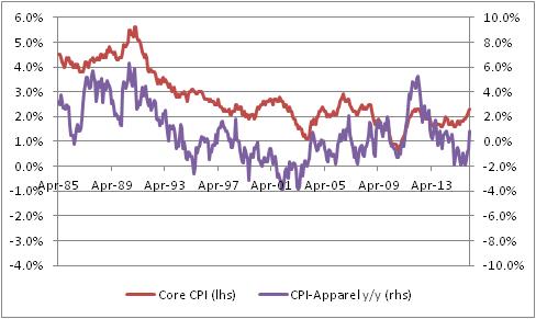
I do have to admit, there is something suggestive about that chart although it is at least somewhat visual since I can’t find a consistent lag structure in the data. But the clear turns do seem to happen first in Apparel, often. Ah, but here is the fun chart. For the next chart, I’ve also taken out Shelter from core inflation, since Shelter especially in recent years has been largely driven by pretty crazy monetary policy, as I have pointed out before many times. (And if you want to read what I think that’s likely to lead to, read my book.) To make it fair, I also removed Apparel itself since once Shelter and Food and Energy are all removed, Apparel is starting to matter.

In this chart, you can start to see a pretty interesting tendency for Apparel to perhaps lead, slightly – and so, perhaps, Ian is right. In this case, I certainly wouldn’t want to bet against him since I think that’s where inflation is going too. I just wasn’t sure that Apparel was a strong part of the argument. (But at the same time, notice the big spike in Apparel inflation in 2012 preceded a rise in ex-housing core, but not a large or sustained rise in ex-housing core).
The table below shows the breakdown of Apparel into its constituent parts. The first column is the category, the second column is the weight (in overall CPI), the third column is the current y/y change, and the fourth column is the previous y/y change.
| Category | Weights | y/y change | prev y/y change |
| Apparel | 3.1% | 0.892% | -0.530% |
| Men’s apparel | 0.63% | -0.445% | 0.483% |
| Boys’ apparel | 0.16% | -0.443% | 1.350% |
| Women’s apparel | 1.04% | 0.230% | -2.127% |
| Girls’ apparel | 0.21% | -1.274% | -2.283% |
| Men’s footwear | 0.21% | 2.854% | -0.461% |
| Boys’ and girls’ footwear | 0.17% | 2.506% | -0.046% |
| Women’s footwear | 0.31% | 0.730% | 0.926% |
| Watches | 0.08% | 8.525% | 0.805% |
| Jewelry | 0.13% | 6.156% | 2.874% |
I look at this to see whether there’s just one category that is having an outsized move; if there were, then we would worry more about one-off effects (say, the rollout of a new kind of women’s blouse that is suddenly all the rage). It is interesting that Men’s apparel and Boys’ apparel decelerated, while most everything else accelerated, but this happens all the time in the Apparel category. Actually, this is a pretty balanced set of sub-indices, for Apparel.
Now, I’m still not 100% sure this isn’t a seasonal-adjustment issue. It could be related to weather, or day count (29 days in February!), or some bottleneck at a port that caused a temporary blip in prices. I want to see a few more months before getting excited like I did in 2012! But we have had a couple of bad core CPI prints, and we also saw pressure in Medical Care so it is fair to say the number of alarm bells has broadened from one (Housing) to several (Housing, Medical Care, Apparel). It is fair to be concerned about price pressures at this point.
Roller Skating in a Buffalo Herd
The ECB fired its “bazooka” today, cutting official rates more into negative territory, increasing QE by another €20bln per month, expanding the range of assets the central bank can buy to now include corporate bonds, and creating a new 4-year program whereby the ECB will loan long-term money to banks at rates that could be negative (based on bank credit extended to corporate and personal borrowers).
My point today is not to opine on the power or wisdom of these policy moves. The main thing I want to observe is this: the inflation market is pricing in what amounts to success for global central banks, with consumer inflation averaging something between 1 and 2 percent per year for the next decade (a bit lower in Japan; a bit higher in the UK). Not only are inflation swaps prices much lower than would be expected from a pure monetarists’ standpoint – but options prices are also very low. The chart below (source: Enduring Investments) shows normalized volatilities[1] over the last five years for a 10-year, 2% year-over-year inflation cap. That is, every year you take a look and see if inflation was over 2%. If it was, then the owner of this option is paid the difference between actual inflation and 2%; if it was not, the owner gets zero. So you get to look ten times at whether inflation has gotten above 2%, and get paid each time it has.

The chart shows that whatever inflation is expected to be, the price to cover the risk that inflation is actually somewhat higher is very low. So, not only is inflation expected to be low, but it is expected to be not volatile either.
Look, we’re talking about bazookas, helicopters…does something not seem right about pricing in very little risk of screwing up?
Whether you believe my thesis in my freshly-released book What’s Wrong With Money?[2] that the likely course of inflation over the next few years is higher and potentially much higher, or you agree with those who think deflation is imminent, shouldn’t we agree that bazookas introduce volatility?
Central banks are attempting to do something that has never been done. Shouldn’t we at least be a teensy bit nervous, as they line up to perform the first-ever quintuple-lutz, that no one has ever landed one before? That no one has ever landed a commercial passenger jet on an aircraft carrier?
Uncertainty is supposed to lower asset values, all else being equal. So even if you think stocks at these levels are “fair,” in an environment with earnings and interest rates where they are now and projected earnings following a certain path, an increase in the volatility of those outcomes should lower the clearing price of those assets since the buyer of the asset (which has positive value) is also assuming the volatility (which has a negative value).
But the market also says that uncertainty right now is low. Yes, the VIX is well off its lows and seems to suggest greater short-term uncertainty (see chart below, source Bloomberg) – but I would argue that the long-term volatility of the economic fundamentals has rarely been this high.

Supposedly you can’t roller skate in a buffalo herd,[3] but we also have never tried to do it. There’s a reason we haven’t tried to do it!
But the Fed, and the rest of the world’s central banks, are not only roller skating in a buffalo herd – the world’s markets seem to be suggesting that investors are sure they’re going to succeed. Regardless of whether you’re optimistic about the outcome, I would argue it’s nearly impossible to be both optimistic and highly confident!
[1] This means something to options traders but can be glossed over by non-options traders. Essentially the point is that you can’t use a regular Black-Scholes model to price options if the strike and/or the forward can have a negative value!
[2] #1 on Amazon in “Economic Inflation,” thanks largely to all of you!
Wimpy’s World
Would you rather have a bar of chocolate today, or one year from today?
Most of us, if we like chocolate, would prefer to have a bar of chocolate today rather than at some point in the future. If you don’t care for chocolate, how about money? Would you rather have $100 today, or $100 next year?
The reason that Wimpy’s “I’ll gladly pay you Tuesday for a hamburger today” ploy doesn’t work is that we would prefer to have the money today compared to the money on Tuesday. If Wimpy wants his burger today, but doesn’t have the money for it, then he must borrow the money and pay that money back on Tuesday. Because of our time preference for money, this will cost Wimpy something extra, as he needs to incentivize us to part with the money today so that he can get his burger now.
This is where it gets weird.
We are now in a Wimpy world. Not only can Wimpy get his burger today, it costs him less if he borrows the money because interest rates are negative. That is, “I’ll gladly pay you less money than the burger costs, and not until Tuesday, for the burger today.” And we are enthusiastically answering, “Sure! Sounds like a great deal!”
This is one weird implication of negative interest rates. If the yield curve was flat at a negative interest rate, it would imply that the further in the future something is, the more valuable it is. A dollar next week is worth more than a dollar today. With negative discount rates, a chocolate bar next year is preferable to a chocolate bar today. And poor Wimpy…being forced to have a hamburger today when a hamburger on Tuesday would be so much better!
It gets even weirder if the yield curve is initially negative but slopes upwards and eventually becomes positive. That implies that discount rates (time preferences) are negative at first, but then flip around and become normal at some point in the future. So there is one day in the future where value is maximized, and it’s less valuable to get money after that date or before that date.
You think this is mere theory, but this is happening internally to derivatives books even as we speak. The models are implying that money later is worth more than money now, because money now costs money to have. And from the standpoint of bank funding, that is absolutely true.
Another strange implication: in general, stocks that do not pay dividends should trade at lower multiples (relative to the firm’s growth) because, being valued only on some terminal cash flow date (when a dividend is paid or when the company is bought out), they’re worth less. But now it is better for a stock to not pay dividends; those dividends have negative value. Technically speaking, this means that companies which cut their dividends should trade at higher prices after the cut.
I can think of more! Ordinarily, if your child enters college the institution will offer you an incentive to pay four years’ tuition at a reduced rate, up front (or at a frozen rate). But, if interest rates are negative, the college should demand a premium if you want to pay up front. Similarly, car companies should insist that you take out a zero-interest-rate loan or else pay a premium if you feel you must pay cash.
In this topsy-turvy world, it is good to be in debt and bad to have a nest egg.
Neighbors appreciate you borrowing a cup of sugar and frown at you when you return it.
Burglars put off burglaries. Baseball teams sign the worst players to the longest deals. Insurance companies pay out life insurance before you die.
And all thanks to negative interest rate policies from your friendly neighborhood central bank. I will thank them tomorrow, when they’ll appreciate it more.
Fed Nonsense and Error Bars
Today’s news was the Employment number. I am not going to talk a lot about the number, since the January jobs number is one of those releases where the seasonal adjustments totally swamp the actual data, and so it has even wider-than-normal error bars. I will discuss error bars more in a moment, but first here is something I do want to point out about the Employment figure. Average Hourly Earnings are now clearly rising. The latest year-on-year number was 2.5%, well above consensus estimates, and last month’s release was revised to 2.7%. So now, the chart of wage growth looks like this.

Of course, I always point out that wages follow inflation, rather than leading it, but since so many people obsess about the wrong inflation metric this may not be readily apparent. But here is Average Hourly Earnings, y/y, versus Median CPI. I have shown this chart before.

The salient point is that whether you are looking at core CPI or PCE or Median CPI, and whether you think wages lead prices or follow prices, this number significantly increases the odds that the Fed raises rates again. Yes, there are lots of reasons the Fed’s intended multi-year tightening campaign is unlikely to unfold, and I am one of those who think that they may already be regretting the first one. But a number like this will tend to convince the hawks among them otherwise.
Speaking of the Fed, last night I attended a speech by Cleveland Fed President Loretta Mester, sponsored by Market News International. Every time I hear a Fed speaker speak, afterwards I want to put my head into a vise to squeeze all of the nonsense out – and last night was no different. Now, Dr. Mester is a classically-trained, highly-accomplished economist with a Ph.D. from Princeton, but I don’t hold that against her. Indeed, credit where credit is due: unlike many such speakers I have heard in the past, Dr. Mester seemed to put more error bars around some of her answers and, in one of the best exchanges, she observed that we won’t really know whether the QE tool is worth keeping in the toolkit until after monetary conditions have returned to normal. That’s unusual; most Fed speakers have long been declaring victory. She is certainly a fan and an advocate of QE, but at least recognizes that the chapter on QE cannot yet be written (although I make what I think is a fair attempt at such a chapter in my book, due out in a month or so).
But the problem with the Federal Reserve boils down to two things. First, like any large institution there is massive groupthink going on. There is little true and significant diversity of opinion. For example there are, for all intents and purposes, no true monetarists left at the Fed who have any voice. Daniel Thornton at the St. Louis Fed was the last one who ever published pieces expressing the important role of money in monetary policy, and he retired a little while back. As another example, it is taken as a given that “transparency” is a good thing, despite the fact that many of the questions posed last night to Dr. Mester boiled down to problems that are actually due to too much transparency. I doubt seriously whether there has ever been a formal discussion, internally, of the connection between increased financial leverage and increased Fed transparency. Many of the problems with “too big to fail” institutions boil down to too much leverage, and a transparent Fed that carefully telegraphs its intentions will tend to increase investor confidence in outcomes and, hence, tend to increase leverage. But I cannot imagine that anyone at the Fed has ever seriously raised the question whether they should be giving less, rather than more, information to the market. It is significantly outside of chapter-and-verse.
The second problem is that the denizens of the Fed overestimate their knowledge and their ability to know certain things that may simply not be knowable. Again, Dr. Mester was a mild exception to this – but very mild. When someone says “We think the overnight rate should normalize more slowly than implied by the Taylor Rule,” but then doesn’t follow that up with an explanation of why you think so, I grow wary. Because economics in the real world, practiced honestly, should produce a lot of “I don’t know” answers. It may be boring, but this is how the question-and-answer with Dr. Mester should have gone:
Q: What do you think inflation will do in 2016?
A: I don’t know. I can tell you my point estimate, but it has really wide error bars.
Q: What do you think short rates will do in 2016?
A: I don’t know. I can tell you my point estimate, but it has really wide error bars.
Q: What do you think the Unemployment Rate will do in 2016?
A: I don’t know. I can tell you my point estimate, but it has really wide error bars.
Q: What do you think the Unemployment Rate will do in 2017?
A: I don’t know. I can tell you my point estimate, but it has really, really wide error bars.
Q: What do you think the consensus is at the Fed about the optimal pace of raising rates?
A: I don’t know. Each person on the Committee has a point estimate, each of which has really wide error bars. Collectively, we have an average that has even wider error bars. We cannot therefore usefully characterize what the path of the short rate will look like. At all.
Indeed, this is part of the problem with transparency. If you are going to be transparent, there is going to be pressure to provide “answers.” But a forecast without an error bar is just a guess. The error bars are what cause a guess to become an estimate. So we get a “dot plot” with a bunch of guesses on it. The actual dot plot, from December, looks like this:

But the dot plot should look more like this, where the error bars are all included.
 Obviously, we would take the latter chart as meaning…correctly…that the Fed really has very little idea of where the funds rate is going to be in a couple of years and cannot convincingly reject the hypothesis that rates will be basically unchanged from here. That’s simultaneously transparent, and very informational, and colossally unhelpful to fast-twitch traders.
And now I can release the vise on my head. Thank you for letting me get the nonsense out.
Zigs and Zags
“The market,” said J.P. Morgan, when asked for his opinion on what the market would do, “will fluctuate.”
Truer words were never spoken, but the depth of the truism as well is interesting. One implication of this observation – that prices will vary – is that the patient investor should mostly ignore noise in the markets. Ben Graham went further; he proposed thinking about a hypothetical “Mister Market,” who every day would offer to buy your stocks or sell you some more. On some days, Mister Market is fearful and offers to sell you stocks at a terrific discount; on other days, he is ebullient and offers to buy your holdings at far more than they are worth. Graham argued that this can only be a positive for an investor who knows the value of the business he holds. He can sell it if Mister Market is paying too much, or buy it if Mister Market is selling it too cheaply.
Graham did not give enough weight to momentum, as opposed to value – the idea that Mister Market might be paying too much today, but if you sell your holdings to him today, then you might miss the opportunity to sell them to him next year for double the stupid price. And, over the last couple of decades, momentum has become far more important to most investors than has value. (I blame CNBC, but that’s a different story).
In either case, the point is important – if you know what you own, and why you own it, and even better if you have an organized framework for thinking about the investment that is time-independent (that is, it doesn’t depend on how you feel today or tomorrow), then the zigs and zags don’t matter much to you in terms of your existing investments.
(As for future investments, young people should prefer declining asset markets, since they will be investing for long periods and should prefer lower prices to buy rather than higher prices; on the other hand, retirees should prefer rising asset prices, since they will be net sellers and should prefer higher prices to lower prices. In practice, everyone seems to like higher prices even though this is not rational in terms of one’s investing life.)
We have recently been experiencing a fair number of zigs, but mostly zags over the last couple of weeks. The stock market is near the last year’s lows – but, it should be noted, it still holds 84% of its gains since March 2009, so it is hardly disintegrating. The dividend yield of the S&P is 2.32%, the highest in some time and once again above 10-year Treasury yields. On the other hand, according to my calculations the expected 10-year return to equities is only about 1.25% more per annum than TIPS yields (0.65% plus inflation, for 10 years), so they are not cheap by any stretch of the imagination. The CAPE is still around 24, which about 50% higher than the historical average. But, in keeping with my point so far: none of these numbers has changed very much in the last couple of weeks. The stock market being down 10%, plus or minus, is a fairly small move from a value perspective (from a momentum perspective, though, it can and has tipped a number of measures).
But here is the more important overarching point to me, right now. I don’t worry about zigs and zags but what I do worry about is the fact that we are approaching the next bear market – whether it is this month, or this year, or next year, we will eventually have a bear market – with less liquidity then when we had the last bear market. Dealers and market-makers have been decimated by regulations and constraints on their deployment of capital, in the name of making them more secure and preventing a “systemic event” in the next calamity. All that means, to me, is that the systemic event will be more distributed. Each investor will face his own systemic event, when he finds the market for his shares is not where he wanted it to be, for the size he needed it to be. This is obviously less of a problem for individual investors. But mutual fund managers, pension fund managers – in short, the people with the big portfolios and the big positions – will have trouble changing their investment stances in a reasonable way (yet another reason to prefer smaller funds and managers, but increasing regulation has also made it very difficult to start and sustain a smaller investment management franchise). Another way to say this is that it is very likely that while the average or median market movement is likely to be similar to what it has been in the past, the tails are likely to be longer than in the past. That is, we may not go from a two-standard-deviation event to a four-standard-deviation event. We may go straight to a six-standard-deviation event.
If market “tails” are likely to be longer than in the past because of (il)liquidity, then the incentive for avoiding those tails is higher. This is true in two ways. First, it creates an incentive for an investor to move earlier, and lighten positions earlier, in a potential downward move in the market. And second, in the context of the Kelly Criterion (see my old article on this topic, here), rising volatility combined with decreased liquidity in general means that at every level of the market, investors should hold more cash than they otherwise would.
I don’t know how far the market will go down, and I don’t really care. I am prepared for “down.” What I care about is how fast.
